By: Jason
Ritchie, Associate Professor of Chemistry
Department
of Chemistry & Biochemistry, The
University of Mississippi
please send comments to jritchie@olemiss.edu
Please download my example gradebook which incorporates examples illustrating
the following topics:
I set-up my gradebook with the standard columns identifying the students name and ID#s. I have them write their ID#s on their tests which helps me find them in the gradebook when I can't read their writing. I just "FIND" their ID#s. Luckily for me, I can download a list of students and ID#s who are enrolled in my class. I took this list and pasted it into Excel and used the "Text to Columns" command found under the "Data" tab to fit this unformatted text to columns in the gradebook.
There are columns for each graded assignment. In this class, I give several quizzes and midterm exams, in addition to a final exam. I told the students that they will be allowed to drop their lowest quiz score and their lowest midterm exam score.
1) How do I get Excelto do standard Statistics?
I use Excelto find the AVERAGE, Standard Deviation (STDEV), the high score (MAX), the low score (MIN), the # of students taking the test (COUNT), the MEDIAN, and the MODE.
Under the column of test scores, I have a series of functions that calculate those statistical values. I then will "Fill Right" (Command-R) when I enter a new set of test scores.
2) How do I get Excelto automatically drop a test score?
In my example gradebook, I have several midterm exams, of which the students get to drop their lowest score. This can be accomplished through Excel's "MIN" function which will find the lowest score in a set of scores. Unfortunately, In my gradebook I like to distinguish between someone who took the test and scored a zero, versus someone who did not take the test. Thus, I leave the space blank for someone who did not take the test. This confuses Excel's "MIN" function somewhat and necessitates the use of an "IF" statement to determine if there are scores for each exam.
So in the "Midterm Total" Column, the function that automatically drops the low score looks like this:
=IF(COUNT(M2,O2,Q2)=3, SUM(M2,O2,Q2)-MIN(M2,O2,Q2), SUM(M2,O2,Q2))
The function starts off with an "IF" statement that asks if there are three midterm test scores. The "COUNT" function looks and sees if there are 3 valid scores (that the student took all 3 tests). If this is true, the "IF" statement executes the next step which is to SUM the 3 tests and subtract the lowest score "MIN". If the student did not take all 3 tests, the IF COUNT=3 test will be false and the function will execute the second command and SUM all three scores. This works because at least one of these will be blank and effectively be zero. These steps are necessary because if a student missed a test, the MIN function will drop their lowest score and not count the missing test as a score.
This function is used to add up and drop the lowest of the quiz scores and the mid-term exam scores.
If you need to drop more than one grade in a set of grades, you can use the SMALL function in Excel. The SMALL function can be used to calculate the nth smallest number in a set of n numbers. Here the command:
=SMALL(M2:P2,1) will return the smallest number in the array M2:P2
while,
=SMALL(M2:P2,2) will return the second smallest number in the array M2:P2
Here I have used the command:
=IF(COUNT(F2:Q2)=12,SUM(F2:Q2)-SMALL(F2:Q2,1)-SMALL(F2:Q2,2),IF(COUNT(F2:Q2)=11,SUM(F2:Q2)-MIN(F2:Q2),SUM(F2:Q2)))
This command, as written, will drop the two lowest quiz scores in a set of 12 quiz scores (F2:Q2). The first command counts the number of scores to see if a student has taken all twelve quizzes, if they have, the sum of the 12 scores is calculated and the lowest and second lowest scores are subtracted. If the student has only taken 11 quizes, the sum is calculated and the smallest score is subtracted. If the student has taken less than 11 quizzes, then the sum of the set is used as their grade.
3) How do I get Excelto automatically calculate a class grade?
In my classes, I either use a standards-based grade approach, or a statistical function to calculate my class grades. I will cover the standards-based approach first.
Standards-based grade calculation:
This is an easy approach if you generally use a ���curve� where a 90% is an A, a 80% is a B, a 70% is a C, 60% is a D, and less than a 60% is an F. The grade calculation is made in two steps. First I add a column that calculates the percentage.
=(V2/430)*100
where "V2" is the "total points" column, and 430 is the total points available. Then use the students percentage score to automatically assign a grade according to the ���curve:
=IF(W3>=90,"A",IF(W3>=80,"B",IF(W3>=70,"C",IF(W3>=60,"D ","F"))))
where W3 is the percentage score. The first IF statement asks if the student has scored higher than 90%, in which case they are awarded an A. The second IF statement asks if the student has scored higher than 80%, in which case they are awarded an B, etc. The last statement says that if a student doesn't fall into any of the first 4 grade categories, they are given an F.
Statistical approach to grade calculation:
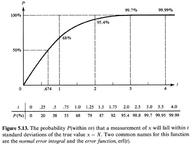
In my case, I define the grades according to the class average and standard
deviation, such that a student who beats the mean by 1 standard deviation
will receive an A (approx. 16% of the normal distribution should beat the
average by one standard deviation.) Students who are above the mean, but
by less than 1 standard deviation will receive a "B". Students who are
up to 1 standard deviation below the mean receive a "C", while students
who are more than 1 standard deviation below the mean will receive a "D"
or an "F". This means that approximately 34% of the students will
receive a "B" with another 34% receiving a "C". Approximately 16%
of the students will receive a "D" or an "F", which is pretty typical in
a freshman chemistry class.
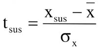
This is accomplished by calculating the function tsus
= [ (student's score) - (average) ] / (standard deviation of average)
I calculate this function in a column next to the "total points" column
called "Weight". The function looks like this:
=(V2-368.1)/31
where "V2" is the "total points" column, 368.1 is the average of the
total points, and 31 is the standard deviation of the average of the total
points.
The grade is then determined from this "Weight" column. I calculate the grade using a complicated "IF" statement that basically determines which category the student falls into. The function looks like this:
=IF(X2>1,"A",IF(X2>0,"B",IF(X2>-1,"C",IF(X2>-1.25,"D","F"))))
where "X2" is the "Weight" column. The IF statement first asks if the student beat the mean by more than 1 standard deviation (X2>1). If this is true, the student is assigned an "A" in that column. If this is false, the statement proceeds to the next argument which asks if the student beat the average (X2>0). If this is true, the student is assigned a "B". Otherwise the IF statement proceeds to the next argument which asks if the student was less than 1 standard deviation below the mean (X2>-1), which if true would result in a grade of "C" being assigned. If false, the IF statement continues to ask if the student was less than 1.25 standard deviations below the mean (X2>-1.25), which if true would result in a grade of "D". If all of the above IF statements result in a false result, the student would be assigned a grade of "F" (that is, the students score is more than 1.25 standard deviations below the mean.
This procedure can be adapted to assign grades based on an arbitrary curve. For instance you might want to calculate a function called "%" which finds the students score as a function of the total points available.
That is %= [ (student score) / (total points available) ] *100
Then you might want to make the IF statement look like this:
=IF(X2>90,"A",IF(X2>80,"B",IF(X2>70,"C",IF(X2>60,"D","F"))))
This way the student will be assigned a grade based on a curve you have determined. In this case a student will a score greater than 90% will receive an "A", while greater than 80% will correspond to a "B", and greater than 70% corresponding to a "C" and so on, with students scoring 60% or less receiving an "F".
Now, I like to keep track of how my grade situation is evolving during the course of the class. So I have set up a table which calculates the #s of grades being assigned and their relative %s. In the table I insert the following function:
=COUNTIF(Y2:Y6, "A")
This function goes down the grade column (Y2:Y6) and counts all the instances of the result "A" and reports in the cell the # of As. This gives a real-time evaluation of the grades being given in the class.